A model of land and housing, part 1: urban growth boundary
How to model upzoning, development charges, LVT, and more

Upzoning increases the supply of housing and reduces prices. But how does this work in a supply and demand model? In this post I’ll walk through a simple general equilibrium model of land and housing, where both the price of land and the price of housing are determined within the model. When zoning is a constraint, the supply of residential land is artificially limited, which restricts housing supply and raises home prices. Upzoning works by relaxing the zoning constraint, which directly increases the supply of housing; as a result, both land prices and housing prices are reduced.
To capture this core mechanism, I use the simplest possible model: a one-time build-out of single-family houses on greenfield land. Developers buy land from farmers and build houses. An urban growth boundary (UGB) is the zoning constraint on the supply of land, and we upzone by expanding the UGB and reallocating land from agricultural to residential. In general, upzoning reallocates land from low- to high-density, so this is analogous to upzoning from detached houses to apartments. (See here for a formal model.)
Setup
We’re building out a new city of single-family houses on undeveloped agricultural land. Each house requires one parcel of land, and an urban growth boundary limits the size of the city by restricting the number of parcels available to build on. We don’t model location, which means assuming all land is in the same location. We also assume all behavior takes place during a single time period. There are three actors in the model: landowners, developers, and homebuyers.
Landowners can farm their land or sell to a developer. All land is the same, so landowners get the same farming payoff. This means that, without an UGB, landowners offer their land to developers at a price equal to this payoff. When developers want more land than the UGB allows, land becomes artificially scarce and the price is bid up above the farming payoff. Now, landowners can sell at an inflated price that includes a scarcity premium.
Developers buy parcels of land and pay fixed construction costs to build houses. We assume developers are competitive, so profits are zero: the revenue from selling a house is equal to construction and land costs. Finally, homebuyers buy houses, demanding a larger total quantity when prices are lower. All houses are the same, and sell for the same price.
From this setup, we get a general equilibrium model of land and housing. In the land market, landowner supply and developer demand determine the price of land; and in the housing market, developer supply and homebuyer demand determine the price of housing.1 Since land is the input used to build housing, developers derive their demand for land from homebuyers’ demand for housing. Similarly, the supply of housing is derived from landowners’ supply of land. Developers are the link between the two markets.
The graphs below show an equilibrium where the UGB is binding.2 In the land market, the supply curve is flat until we reach the UGB, where it becomes vertical. We say that landowners are ‘perfectly elastic’, meaning they will offer any quantity at the same price (here, the farming payoff of 40). The UGB makes supply ‘perfectly inelastic:’ no matter how much prices rise, landowners cannot sell a larger quantity of land. The demand curve intersects the supply curve where it is vertical, which means the UGB is a constraint on residential land; if we could expand the UGB, developers would buy more land.
Because the UGB is binding, residential land is a fixed factor, so its price is determined as a residual, as the housing price minus construction costs. Land is artificially scarce and includes a scarcity premium, making it more expensive than agricultural land. Here, the residential land price is bid up to 100 and the farming payoff is 40, so the scarcity premium is 100 - 40 = 60. When zoning is not a constraint, residential and agricultural land sells for the same price, and the scarcity premium is zero.
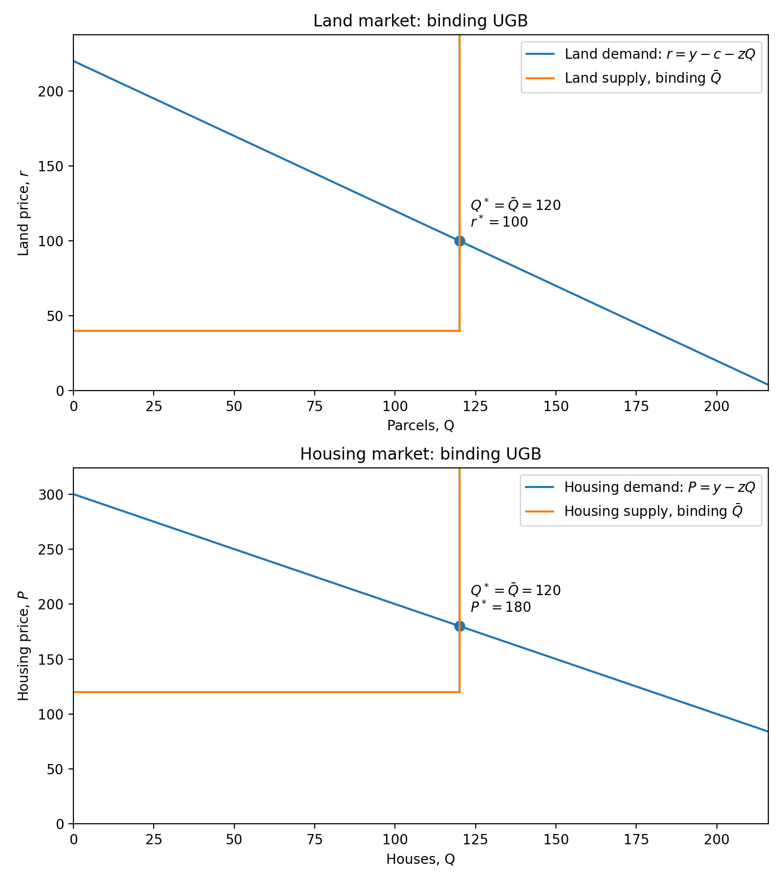
In the housing market, we assume that homebuyers have downward-sloping demand: at lower prices, they are willing to buy a larger quantity of houses. Below the UGB, the housing supply curve is horizontal, and we calculate it by adding construction costs (80) to the land supply curve; developers build houses by paying land and construction costs (40 + 80 = 120). Because landowners are perfectly elastic suppliers, so too are developers. But once the UGB binds, the supply curve contains the scarcity premium and becomes vertical. (Similarly, the land demand curve is calculated as the housing demand curve minus construction costs.)
With a binding UGB, housing supply is constrained, pushing up house prices. If we could expand the UGB, we would move down the demand curve, increasing quantity and reducing housing prices.
Upzoning: expanding the UGB
So let’s expand the growth boundary and see what happens. Upzoning means shifting the land supply curve to the right, because we’re allowing more land to be used for housing. Each house uses one parcel of land, so more land means that the housing supply curve also shifts right, leading to lower housing prices. In the land market, increased supply leads to lower land prices, decreasing the scarcity premium on residential land.
In the graphs below, we expand the UGB from 120 parcels to 155. This reduces housing prices from 180 to 145, land prices from 100 to 65, and the scarcity premium from 60 to 25. So the constraint is still binding, but not as stringently.
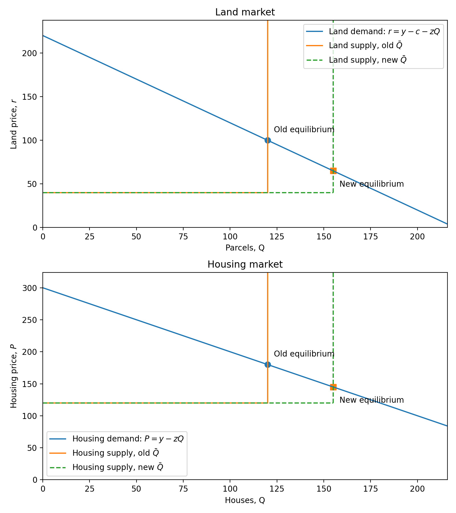
Here upzoning reduces the land price of existing residential land. This is the cross-parcel effect, where increasing the supply of land (by 35 parcels) reduces the price of the original 120 residential parcels. When land is constrained and priced as a residual, lower housing prices translate to lower residual land values. (Generally, upzoning from low- to high-density reduces the price of existing high-density land.)
In contrast, the own-parcel effect is the increase in value for the 35 newly upzoned parcels. Initially, these were worth the farming payoff of 40. Upzoning them to residential increases their value to the new land price of 65, for a gain of 25. This is a windfall gain for those landowners, but the increase in price is not relevant to developers, since the land wasn’t even available to them when it was zoned for farming. All that matters for the housing market is that the stock of residential land is larger.
Also note that if we upzoned even more, by increasing the UGB to 180 parcels (or more), then the scarcity premium would be reduced to 0. Residential land would be so abundant that it would sell for the same price as agricultural land. In this case, the own-parcel effect is also 0: with no scarcity premium, agricultural landowners do not benefit from acquiring development rights. And when land is abundant, any additional upzonings have no effect on land prices.
This is the YIMBY endgame: upzoning so much that zoning is no longer a constraint, which achieves the maximum reduction in housing prices. In general, the policy goal is to have equal land prices for otherwise similar low- and high-density land.
Do higher construction costs increase housing prices?
One counterintuitive argument is that higher construction costs do not lead to higher housing prices, because market prices are fixed and higher costs just reduce land values. With our general equilibrium model, we can sort this out. When the UGB is not binding, prices are set by marginal costs, so higher costs lead to higher prices. But when the UGB is a binding constraint, prices are set by scarcity, not marginal costs. In this case, a small increase in costs reduces the scarcity premium on land without affecting housing prices, as demonstrated below. Costs increase by 40, and land prices fall by 40. The housing supply curve shifts up with no effect, since we’re eating into the scarcity premium.3
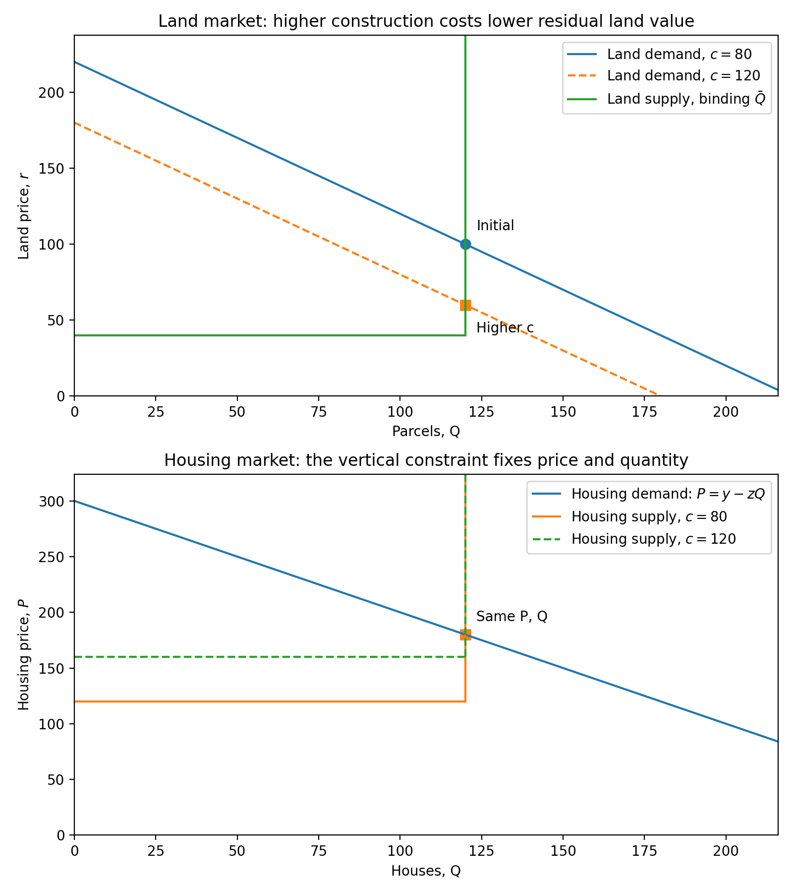
So whether costs affect housing prices depends on whether the zoning constraint is binding. If costs increase enough, developers don’t want to build as many houses and the UGB stops binding. Then we’re back in the scenario where construction costs are passed through to housing prices.
Do development taxes increase housing prices?
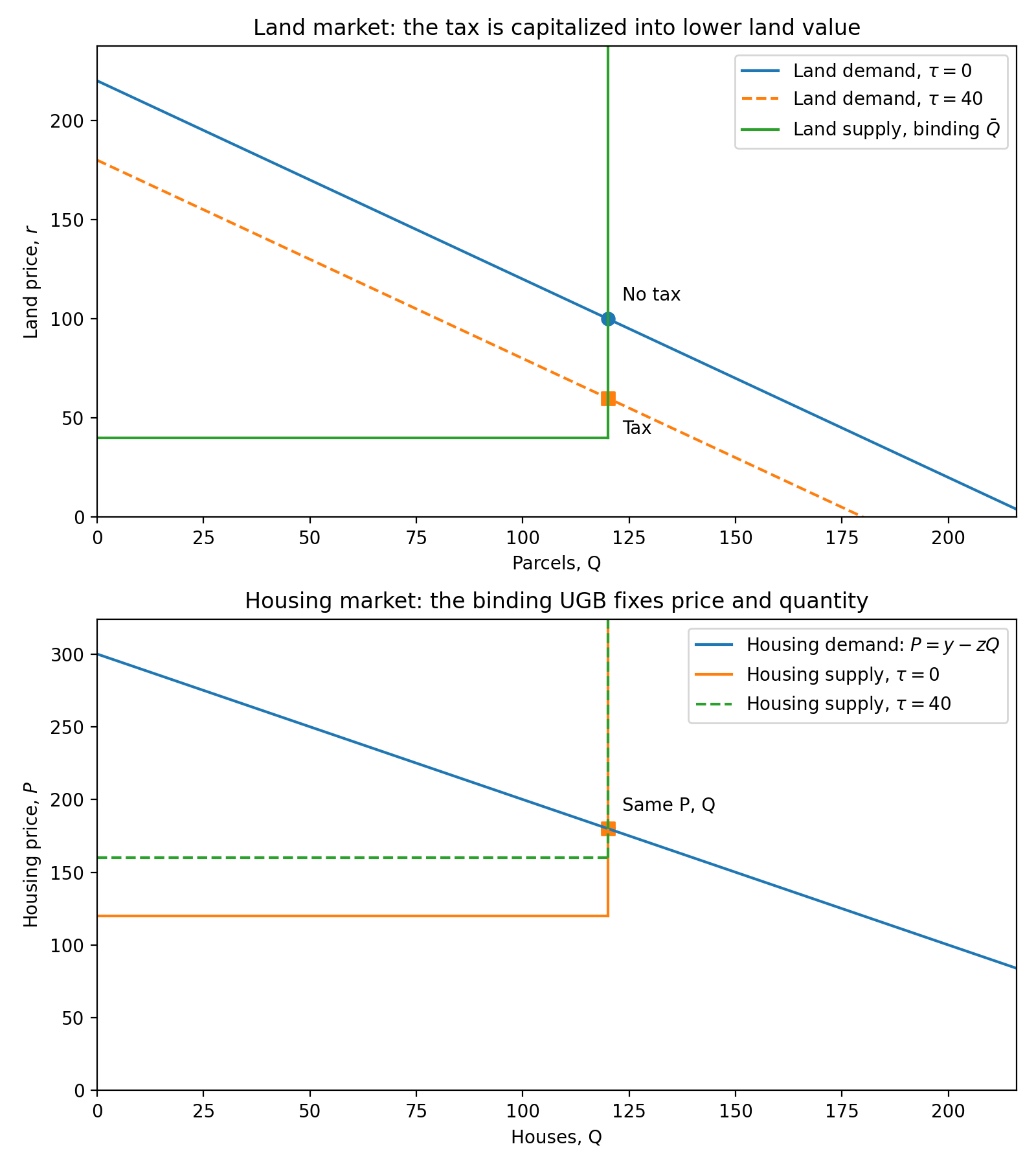
If we tax developers for building houses, do we get higher housing prices or lower land prices? As with construction costs, it depends on whether the UGB is a binding constraint. First, a primer on tax incidence. Even though developers are charged the tax when they buy land (they bear the ‘statutory incidence’), they can pass on the tax to landowners or homebuyers, due to our assumption of making zero profit. So the tax is actually paid by landowners or homebuyers (they bear the ‘economic incidence’), and this is determined by who is more responsive to price changes (i.e., more price-elastic).
When the UGB is binding, landowners cannot supply more land, no matter how high prices are. Here landowners are unresponsive to prices (perfectly inelastic), and developers can pass on the tax to landowners by paying lower land prices. And when the UGB is slack, landowners are perfectly elastic, since they offer any quantity of parcels at the farming payoff. Here, landowners are more price responsive than homebuyers, so developers can pass on the tax to homebuyers by increasing housing prices.
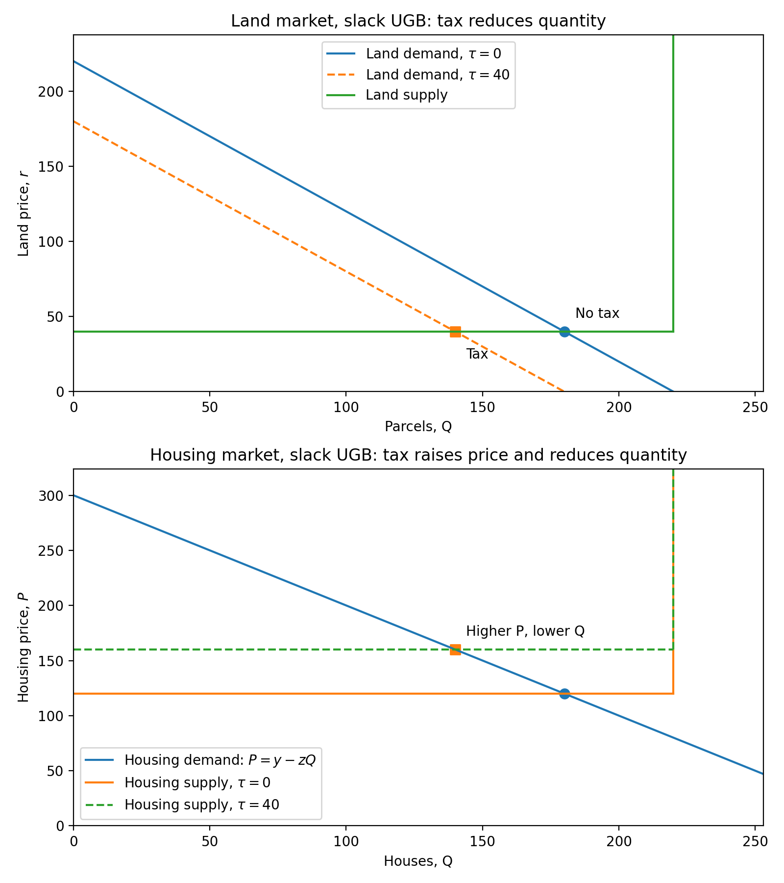
The graphs below show a non-binding UGB. When zoning is not a constraint, the tax reduces developers’ demand for land, shifting the demand curve down. The tax acts like a cost, shifting the housing supply curve up, which reduces the quantity and increases the price of housing.
Next let’s see the binding UGB case. Here the tax also reduces demand for land, but because the zoning constraint makes landowners inelastic, developers can reduce their land payment without affecting the quantity of parcels. The housing supply curve shifts up, but this doesn’t change anything. Essentially, the tax comes out of the scarcity premium with no effect on housing prices, exactly the same as the cost increase above. If the tax is large enough, then the housing supply curve shifts up and the UGB stops binding, and we switch back to the case above where the tax increases house prices.
The political incentives here can be quite perverse. If the government wants to raise revenue while appearing to tax landowner windfalls, they are incentivized to impose an UGB, thereby creating a scarcity premium to tax. But as we saw when studying upzoning, the zoning constraint creates a scarcity premium only by raising housing prices! So even though the tax itself doesn’t affect the housing market, the combination of restrictive zoning and development taxes does result in higher prices. Even if the tax revenue is used to fund subsidized housing, the best case scenario is that housing prices fall back to their original level. We cannot improve affordability by first creating scarcity.
We can also interpret a development tax as value capture from upzoning, taxing the ‘land lift’ on upzoned land that increases in value. Initially, the UGB is set at zero parcels and no development is allowed; land is priced at the farming payoff of 40. Then we upzone by expanding the UGB to 120 parcels, and the upzoned land increases in price to 100. We’ve created a scarcity premium of 100 - 40 = 60 that the government can tax.
But the scarcity premium exists only because we did a limited upzoning. If we had upzoned to 180 parcels, the scarcity premium would be zero and the government would have nothing to tax. Since the UGB isn’t binding, any tax would fall on homebuyers, raising prices. So a government that depends on revenue from development taxes is incentivized to do limited upzonings to create a taxable scarcity premium. A government that cared about housing affordability would upzone as much as possible to minimize housing prices.
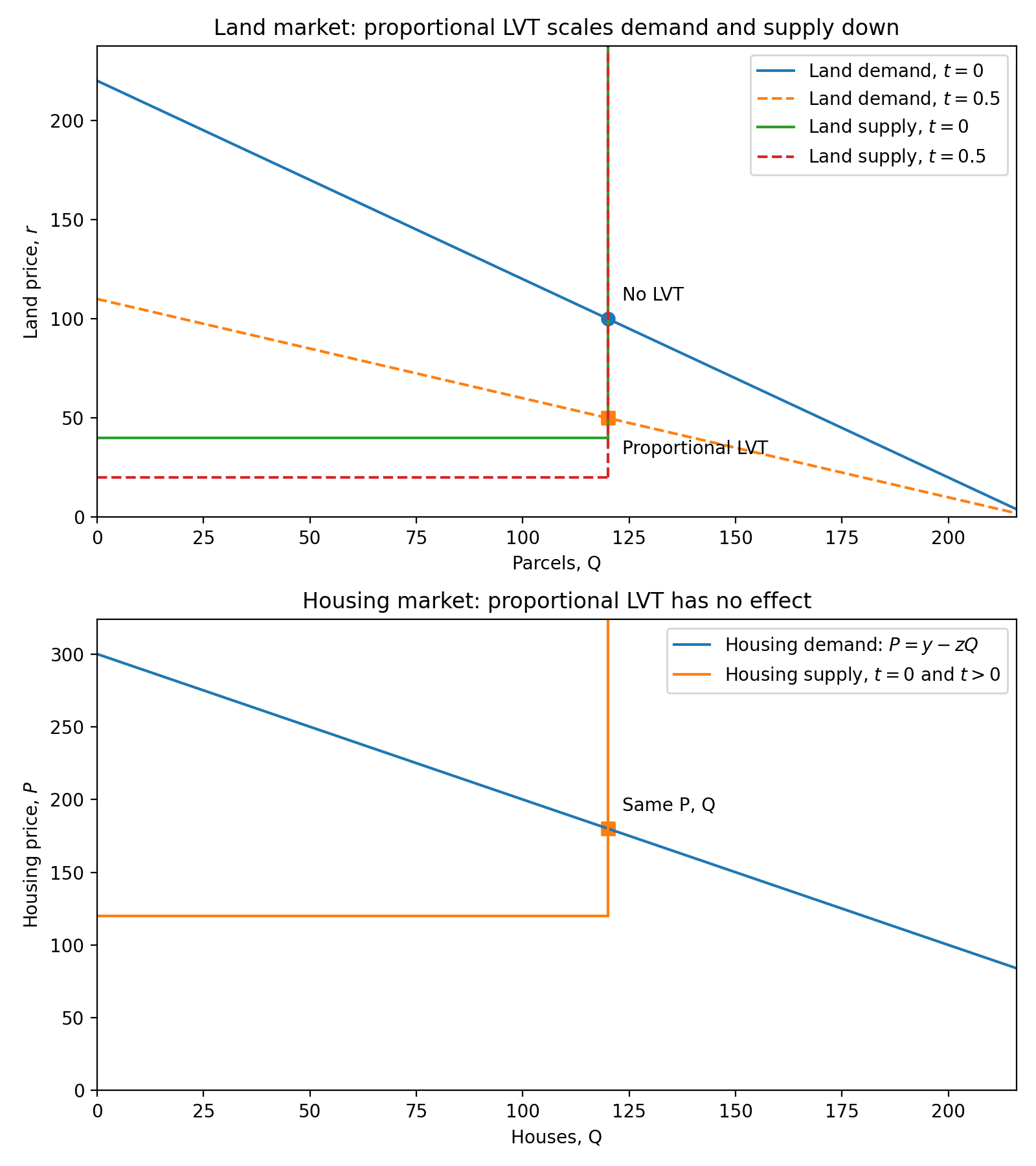
Land value taxes don’t affect housing prices
In contrast to development taxes, a land value tax does not affect housing prices. While a development tax is imposed only when a development occurs, a land value tax is charged to the landowner unconditionally, even when no housing is built. This is the key difference that makes land value taxes non-distortionary and hence a favorite of economists. Landowners are taxed on their farming payoff, so even though a developer has to pay a tax to own land, they also pay lower land prices, so the effects cancel out.
The graphs below show a 50% proportional tax on the value of the land. The demand curve for land shifts down, same as the development tax. But now the land supply curve also shifts down, reflecting that landowners are taxed on their outside option. Since both curves shift, there’s no effect on the quantity of land, and the housing market is unchanged. Land prices fall and housing prices are the same. When the UGB is binding, an LVT reduces the scarcity premium on land, so it can be used as a value capture mechanism.
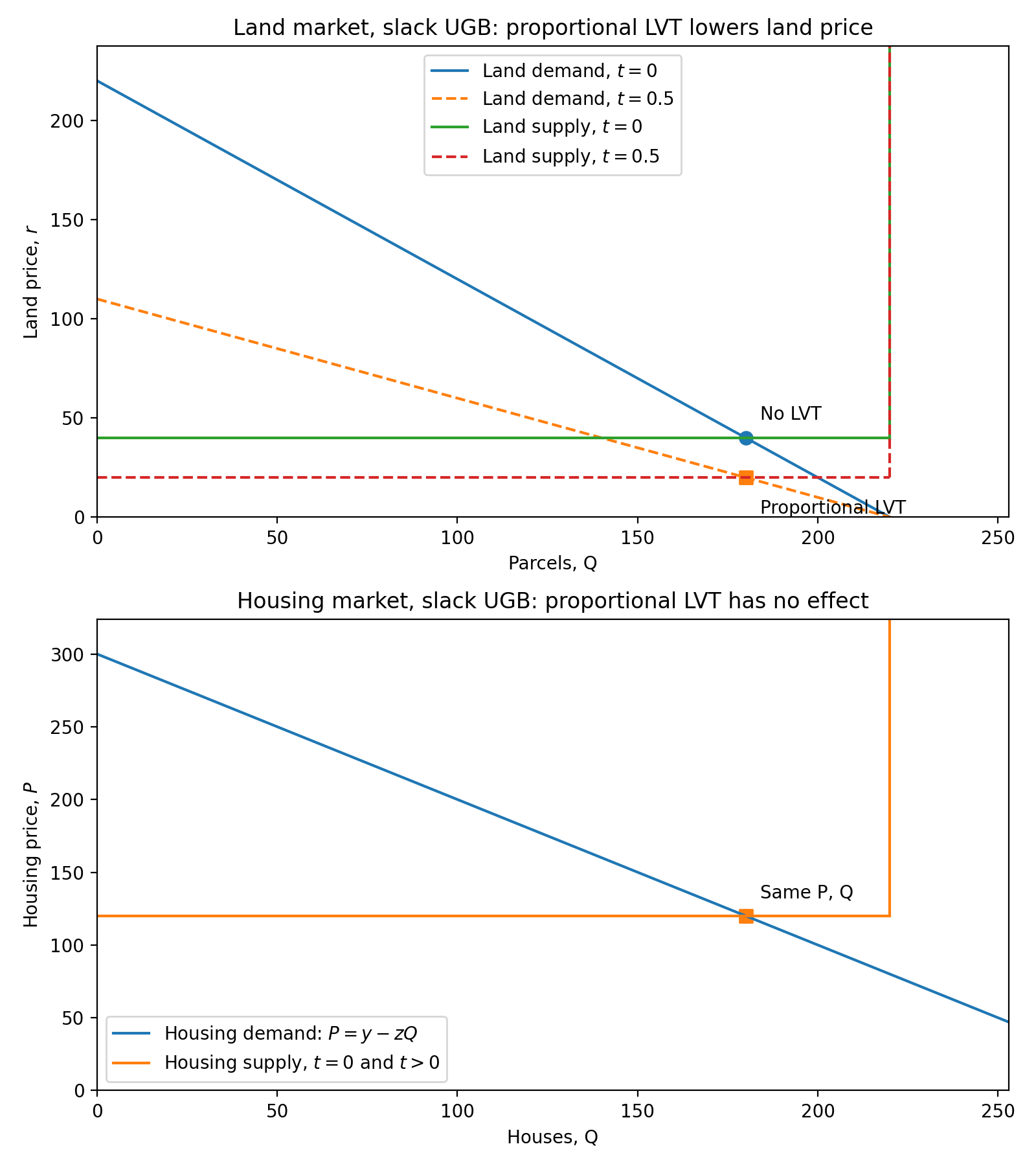
An LVT also has no effect on housing prices when the UGB is slack. Again, since both curves shift down in the land market, there’s no effect on quantity, and hence no change in the housing market.
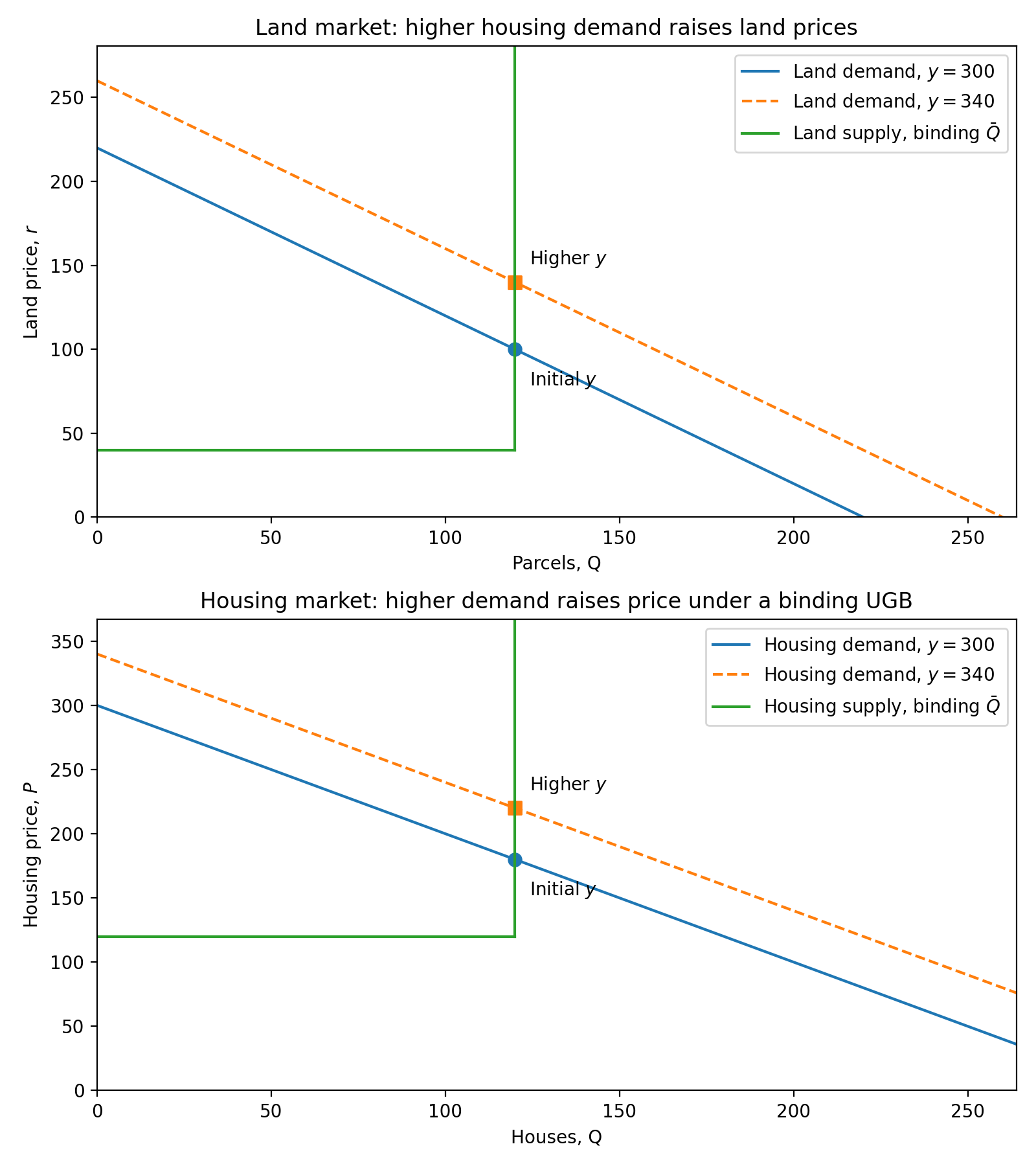
Land prices are driven by housing demand
Finally, let’s consider the argument that upzoning is the main factor driving up land prices. While it is true that upzoning can have a positive own-parcel effect (because residential land is priced above agricultural land), rising land prices are generally driven by increased housing demand.
When the UGB is binding, land prices are directly determined by the level of housing demand (via the demand curve intercept y). Shifting up the housing demand curve raises house prices, which also increases developer demand for land, thereby increasing land prices. So it makes sense that a city with growing demand will have higher housing and land prices.
We can confirm this by looking at a natural experiment where upzoning isn’t allowed. First Shaughnessy, a heritage-protected mansion neighborhood in Vancouver, has seen a 5x increase in land values even without any upzonings. This suggests that housing demand has increased 5x in Vancouver.
Conclusion
A simple supply and demand model of land and housing can explain how upzoning works, whether increased construction costs and taxes lead to higher housing prices, and how housing demand drives land prices. This model assumes one housing good, one zone, and one location, as the simplest model that captures how upzoning works. In future posts, I will extend it to have two zones (house- and apartment-zoning), two housing goods (houses and apartments), and two locations (city and suburb).
See here for the formal model.
What makes it a general equilibrium model is that prices in both markets are determined within the model. A partial equilibrium model would take, for example, housing prices as fixed (determined outside of the model) and derive land prices.
Parameters: farming payoff = 40, construction cost = c = 80, UGB = Q_bar = 120, y = 300, z =1.
Another angle: land is priced residually as housing prices minus construction costs, so when housing prices are determined by the constraint, an increase in costs just reduces residual land value.